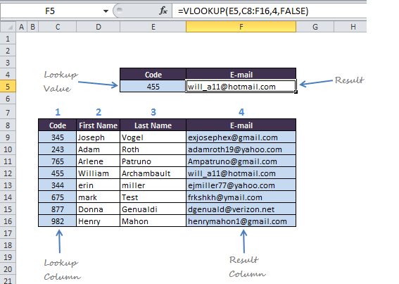
In this tutorial we are going to explain you how you can use the VLOOKUP Function in Microsoft Excel
Purpose
When you need to find things from a big table or a range by row. VLOOKUP searches for a value in the first column of a table. At the match row, it retrieves a value from the specified column.
Return Value
The matched value from a table.
Syntax
=VLOOKUP (lookup_value, table_array, col_index_num, [range_lookup])
Arguments
- lookup_value - The value to look for in the first column of a table.
- table_array - The table from which to retrieve a value.
- col_index_num - The column in the table from which to retrieve a value.
- range_lookup - [optional] TRUE or 1 = approximate match (default). FALSE or 0 = exact match.
Note: Recommended [range_lookup] as 0 or FALSE, as mostly required exact output.
Simplifying above Syntax and Arguments
=VLOOKUP(ItemToFind,RangeToLookIn,ColumnToPickFrom,SortedOrUnsorted)
The
ItemToFind is a single item specified by the user.
The
RangeToLookIn is the range of data with the row headings at the left
hand side.
The ColumnToPickFrom is how far across the table the
function should look to pick from.
The Sorted/Unsorted is whether
the column headings are sorted. TRUE for yes, FALSE for no.
Note: Recommended [range_lookup] as 0 or FALSE, as mostly
required exact output.

No comments:
Post a Comment